What Is Modeling as It Relates to Science and or Math

Description of a organization using mathematical concepts and linguistic communication

A mathematical model is a description of a system using mathematical concepts and language. The procedure of developing a mathematical model is termed mathematical modeling. Mathematical models are used in the natural sciences (such every bit physics, biology, globe science, chemistry) and engineering disciplines (such as estimator science, electrical technology), as well equally in non-physical systems such as the social sciences (such as economic science, psychology, sociology, political science). The use of mathematical models to solve bug in business organisation or military operations is a large office of the field of operations enquiry. Mathematical models are also used in music,^[one] linguistics,^[2] and philosophy (for example, intensively in analytic philosophy).

A model may assist to explain a organization and to study the effects of dissimilar components, and to brand predictions about behavior.

Elements of a mathematical model [edit]

Mathematical models tin can have many forms, including dynamical systems, statistical models, differential equations, or game theoretic models. These and other types of models tin can overlap, with a given model involving a diverseness of abstract structures. In general, mathematical models may include logical models. In many cases, the quality of a scientific field depends on how well the mathematical models adult on the theoretical side agree with results of repeatable experiments. Lack of agreement between theoretical mathematical models and experimental measurements often leads to important advances as ameliorate theories are developed.

In the physical sciences, a traditional mathematical model contains most of the following elements:

1. Governing equations
2. Supplementary sub-models
   1. Defining equations
   2. Constitutive equations
3. Assumptions and constraints
   1. Initial and boundary conditions
   2. Classical constraints and kinematic equations

Classifications [edit]

Mathematical models are ordinarily composed of relationships and variables. Relationships can exist described by operators, such as algebraic operators, functions, differential operators, etc. Variables are abstractions of organization parameters of involvement, that tin can be quantified. Several nomenclature criteria can be used for mathematical models according to their structure:

• Linear vs. nonlinear: If all the operators in a mathematical model exhibit linearity, the resulting mathematical model is defined as linear. A model is considered to be nonlinear otherwise. The definition of linearity and nonlinearity is dependent on context, and linear models may have nonlinear expressions in them. For case, in a statistical linear model, information technology is assumed that a human relationship is linear in the parameters, but it may exist nonlinear in the predictor variables. Similarly, a differential equation is said to exist linear if information technology tin can be written with linear differential operators, but it tin withal have nonlinear expressions in it. In a mathematical programming model, if the objective functions and constraints are represented entirely past linear equations, then the model is regarded every bit a linear model. If i or more than of the objective functions or constraints are represented with a nonlinear equation, then the model is known as a nonlinear model.
  Linear construction implies that a problem tin can be decomposed into simpler parts that tin exist treated independently and/or analyzed at a dissimilar scale and the results obtained will remain valid for the initial problem when recomposed and rescaled.
  Nonlinearity, even in fairly simple systems, is frequently associated with phenomena such every bit anarchy and irreversibility. Although in that location are exceptions, nonlinear systems and models tend to be more than hard to study than linear ones. A common arroyo to nonlinear problems is linearization, but this can be problematic if one is trying to study aspects such as irreversibility, which are strongly tied to nonlinearity.
• Static vs. dynamic: A dynamic model accounts for time-dependent changes in the state of the system, while a static (or steady-state) model calculates the system in equilibrium, and thus is time-invariant. Dynamic models typically are represented by differential equations or difference equations.
• Explicit vs. implicit: If all of the input parameters of the overall model are known, and the output parameters can be calculated by a finite series of computations, the model is said to exist explicit. Simply sometimes it is the output parameters which are known, and the corresponding inputs must be solved for past an iterative procedure, such equally Newton's method or Broyden'south method. In such a case the model is said to be implicit. For example, a jet engine's physical properties such equally turbine and nozzle throat areas tin can be explicitly calculated given a design thermodynamic cycle (air and fuel catamenia rates, pressures, and temperatures) at a specific flight condition and power setting, but the engine's operating cycles at other flying conditions and power settings cannot exist explicitly calculated from the constant concrete backdrop.
• Detached vs. continuous: A discrete model treats objects as detached, such equally the particles in a molecular model or u.s. in a statistical model; while a continuous model represents the objects in a continuous fashion, such as the velocity field of fluid in pipe flows, temperatures and stresses in a solid, and electrical field that applies continuously over the entire model due to a point charge.
• Deterministic vs. probabilistic (stochastic): A deterministic model is i in which every set of variable states is uniquely determined past parameters in the model and by sets of previous states of these variables; therefore, a deterministic model always performs the aforementioned way for a given gear up of initial conditions. Conversely, in a stochastic model—commonly called a "statistical model"—randomness is present, and variable states are not described by unique values, only rather by probability distributions.
• Deductive, inductive, or floating: A deductive model is a logical structure based on a theory. An inductive model arises from empirical findings and generalization from them. The floating model rests on neither theory nor observation, just is merely the invocation of expected structure. Application of mathematics in social sciences outside of economics has been criticized for unfounded models.^[3] Application of catastrophe theory in science has been characterized equally a floating model.^[4]
• Strategic vs non-strategic Models used in game theory are unlike in a sense that they model agents with incompatible incentives, such as competing species or bidders in an auction. Strategic models assume that players are autonomous determination makers who rationally choose deportment that maximize their objective function. A fundamental challenge of using strategic models is defining and computing solution concepts such equally Nash equilibrium. An interesting belongings of strategic models is that they divide reasoning almost rules of the game from reasoning well-nigh behavior of the players.^[5]

Construction [edit]

In business and engineering, mathematical models may exist used to maximize a sure output. The system under consideration volition require certain inputs. The system relating inputs to outputs depends on other variables too: conclusion variables, state variables, exogenous variables, and random variables.

Decision variables are sometimes known as independent variables. Exogenous variables are sometimes known as parameters or constants. The variables are not independent of each other as the country variables are dependent on the conclusion, input, random, and exogenous variables. Furthermore, the output variables are dependent on the country of the system (represented by the land variables).

Objectives and constraints of the system and its users can exist represented as functions of the output variables or state variables. The objective functions will depend on the perspective of the model'due south user. Depending on the context, an objective office is likewise known as an alphabetize of operation, as it is some measure of interest to the user. Although in that location is no limit to the number of objective functions and constraints a model tin can accept, using or optimizing the model becomes more than involved (computationally) as the number increases.

For example, economists often apply linear algebra when using input-output models. Complicated mathematical models that take many variables may exist consolidated past use of vectors where one symbol represents several variables.

A priori information [edit]

To analyse something with a typical "blackness box approach", only the beliefs of the stimulus/response volition be accounted for, to infer the (unknown) box. The usual representation of this black box arrangement is a data flow diagram centered in the box.

Mathematical modeling issues are often classified into blackness box or white box models, co-ordinate to how much a priori information on the system is available. A black-box model is a system of which there is no a priori information available. A white-box model (also called drinking glass box or articulate box) is a system where all necessary data is available. Practically all systems are somewhere between the blackness-box and white-box models, so this concept is useful only as an intuitive guide for deciding which arroyo to take.

Usually it is preferable to use as much a priori information as possible to brand the model more accurate. Therefore, the white-box models are normally considered easier, because if you accept used the information correctly, then the model will behave correctly. Oft the a priori data comes in forms of knowing the type of functions relating dissimilar variables. For case, if we make a model of how a medicine works in a human being system, we know that usually the amount of medicine in the blood is an exponentially decomposable function. But nosotros are still left with several unknown parameters; how rapidly does the medicine amount decay, and what is the initial amount of medicine in blood? This example is therefore not a completely white-box model. These parameters have to be estimated through some means before one tin use the model.

In blackness-box models one tries to guess both the functional course of relations between variables and the numerical parameters in those functions. Using a priori information we could end upwardly, for example, with a set up of functions that probably could describe the system adequately. If there is no a priori information we would try to use functions every bit general as possible to comprehend all different models. An oft used approach for blackness-box models are neural networks which usually do not brand assumptions well-nigh incoming data. Alternatively the NARMAX (Nonlinear AutoRegressive Moving Average model with eXogenous inputs) algorithms which were adult as part of nonlinear system identification^[6] can be used to select the model terms, determine the model construction, and estimate the unknown parameters in the presence of correlated and nonlinear noise. The advantage of NARMAX models compared to neural networks is that NARMAX produces models that can exist written down and related to the underlying procedure, whereas neural networks produce an approximation that is opaque.

Subjective information [edit]

Sometimes it is useful to incorporate subjective information into a mathematical model. This can be done based on intuition, experience, or expert opinion, or based on convenience of mathematical class. Bayesian statistics provides a theoretical framework for incorporating such subjectivity into a rigorous analysis: we specify a prior probability distribution (which can be subjective), and then update this distribution based on empirical information.

An example of when such approach would be necessary is a state of affairs in which an experimenter bends a money slightly and tosses information technology once, recording whether it comes upwards heads, and is so given the chore of predicting the probability that the side by side flip comes upwardly heads. Afterwards angle the coin, the true probability that the coin will come up heads is unknown; so the experimenter would need to make a conclusion (perhaps by looking at the shape of the coin) well-nigh what prior distribution to utilise. Incorporation of such subjective data might be important to get an accurate estimate of the probability.

Complexity [edit]

In general, model complication involves a merchandise-off between simplicity and accuracy of the model. Occam's razor is a principle particularly relevant to modeling, its essential thought beingness that among models with roughly equal predictive power, the simplest ane is the most desirable. While added complexity usually improves the realism of a model, information technology can brand the model difficult to understand and clarify, and tin also pose computational problems, including numerical instability. Thomas Kuhn argues that as science progresses, explanations tend to get more circuitous before a paradigm shift offers radical simplification.^[7]

For example, when modeling the flying of an aircraft, we could embed each mechanical part of the aircraft into our model and would thus acquire an almost white-box model of the system. However, the computational toll of adding such a huge amount of detail would effectively inhibit the usage of such a model. Additionally, the uncertainty would increment due to an overly circuitous system, because each separate part induces some amount of variance into the model. It is therefore usually appropriate to brand some approximations to reduce the model to a sensible size. Engineers often can accept some approximations in order to get a more robust and unproblematic model. For instance, Newton'due south classical mechanics is an approximated model of the real world. Still, Newton'south model is quite sufficient for most ordinary-life situations, that is, every bit long as particle speeds are well beneath the speed of light, and nosotros study macro-particles only.

Notation that improve accuracy does not necessarily mean a better model. Statistical models are prone to overfitting which ways that a model is fitted to data also much and it has lost its ability to generalize to new events that were not observed before.

Training and tuning [edit]

Any model which is not pure white-box contains some parameters that tin be used to fit the model to the organization it is intended to depict. If the modeling is done past an artificial neural network or other machine learning, the optimization of parameters is called training, while the optimization of model hyperparameters is chosen tuning and frequently uses cantankerous-validation.^[8] In more conventional modeling through explicitly given mathematical functions, parameters are often determined past curve fitting ^{[ citation needed ]}.

Model evaluation [edit]

A crucial part of the modeling procedure is the evaluation of whether or not a given mathematical model describes a system accurately. This question can be difficult to reply as it involves several different types of evaluation.

Fit to empirical data [edit]

Ordinarily, the easiest office of model evaluation is checking whether a model fits experimental measurements or other empirical information. In models with parameters, a mutual approach to test this fit is to split the data into two disjoint subsets: preparation data and verification data. The grooming data are used to estimate the model parameters. An authentic model will closely match the verification data fifty-fifty though these information were not used to set the model's parameters. This practice is referred to every bit cross-validation in statistics.

Defining a metric to measure out distances between observed and predicted information is a useful tool for assessing model fit. In statistics, conclusion theory, and some economic models, a loss part plays a similar role.

While it is rather straightforward to test the appropriateness of parameters, it tin be more hard to examination the validity of the general mathematical form of a model. In full general, more mathematical tools have been developed to test the fit of statistical models than models involving differential equations. Tools from nonparametric statistics can sometimes be used to evaluate how well the data fit a known distribution or to come up up with a general model that makes merely minimal assumptions nearly the model's mathematical form.

Scope of the model [edit]

Assessing the scope of a model, that is, determining what situations the model is applicable to, can be less straightforward. If the model was constructed based on a set of information, 1 must determine for which systems or situations the known data is a "typical" fix of data.

The question of whether the model describes well the properties of the arrangement betwixt information points is chosen interpolation, and the same question for events or information points outside the observed data is called extrapolation.

As an example of the typical limitations of the telescopic of a model, in evaluating Newtonian classical mechanics, we can note that Newton fabricated his measurements without avant-garde equipment, so he could not mensurate properties of particles travelling at speeds close to the speed of light. Likewise, he did non measure out the movements of molecules and other small-scale particles, merely macro particles only. It is so non surprising that his model does not extrapolate well into these domains, fifty-fifty though his model is quite sufficient for ordinary life physics.

Philosophical considerations [edit]

Many types of modeling implicitly involve claims about causality. This is usually (but non always) true of models involving differential equations. As the purpose of modeling is to increment our understanding of the world, the validity of a model rests non only on its fit to empirical observations, but besides on its power to extrapolate to situations or data beyond those originally described in the model. One can recollect of this as the differentiation between qualitative and quantitative predictions. One can also fence that a model is worthless unless it provides some insight which goes across what is already known from direct investigation of the phenomenon being studied.

An case of such criticism is the argument that the mathematical models of optimal foraging theory do non offer insight that goes beyond the common-sense conclusions of evolution and other bones principles of environmental.^[nine]

Significance in the natural sciences [edit]

Mathematical models are of corking importance in the natural sciences, especially in physics. Physical theories are nigh invariably expressed using mathematical models.

Throughout history, more and more accurate mathematical models accept been developed. Newton'south laws accurately describe many everyday phenomena, but at certain limits theory of relativity and quantum mechanics must be used.

It is mutual to use idealized models in physics to simplify things. Massless ropes, point particles, ideal gases and the particle in a box are among the many simplified models used in physics. The laws of physics are represented with simple equations such every bit Newton'southward laws, Maxwell's equations and the Schrödinger equation. These laws are a basis for making mathematical models of real situations. Many real situations are very complex and thus modeled approximate on a estimator, a model that is computationally feasible to compute is made from the basic laws or from judge models fabricated from the basic laws. For instance, molecules tin be modeled past molecular orbital models that are approximate solutions to the Schrödinger equation. In engineering, physics models are oftentimes made by mathematical methods such as finite element analysis.

Different mathematical models use different geometries that are not necessarily accurate descriptions of the geometry of the universe. Euclidean geometry is much used in classical physics, while special relativity and general relativity are examples of theories that use geometries which are not Euclidean.

Some applications [edit]

Often when engineers clarify a system to be controlled or optimized, they apply a mathematical model. In assay, engineers can build a descriptive model of the system as a hypothesis of how the arrangement could work, or try to approximate how an unforeseeable result could affect the organization. Similarly, in control of a system, engineers can try out different control approaches in simulations.

A mathematical model usually describes a system by a set of variables and a gear up of equations that plant relationships between the variables. Variables may be of many types; real or integer numbers, boolean values or strings, for example. The variables represent some properties of the system, for example, the measured system outputs often in the class of signals, timing data, counters, and event occurrence . The actual model is the set of functions that describe the relations between the different variables.

Examples [edit]

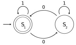
• One of the pop examples in computer science is the mathematical models of various machines, an example is the deterministic finite automaton (DFA) which is defined every bit an abstract mathematical concept, but due to the deterministic nature of a DFA, it is implementable in hardware and software for solving various specific bug. For example, the following is a DFA Grand with a binary alphabet, which requires that the input contains an even number of 0s:

M = (Q, Σ, δ, q ₀, F) where

• Q = {S _i, S ₂},
• Σ = {0, ane},
• q₀ = S ₁,
• F = {S ₁}, and
• δ is divers by the following state transition table:

The country S ₁ represents that at that place has been an even number of 0s in the input so far, while S ₂ signifies an odd number. A one in the input does non change the country of the automaton. When the input ends, the land will show whether the input contained an even number of 0s or not. If the input did comprise an even number of 0s, M will stop in state S ₁, an accepting state, and then the input cord will be accepted.

The linguistic communication recognized by Chiliad is the regular linguistic communication given by the regular expression 1*( 0 (1*) 0 (1*) )*, where "*" is the Kleene star, e.g., 1* denotes whatsoever non-negative number (perchance zero) of symbols "1".

${\displaystyle -{\frac {\mathrm {d} ^{2}\mathbf {r} (t)}{\mathrm {d} t^{2}}}grand={\frac {\partial V[\mathbf {r} (t)]}{\partial x}}\mathbf {\hat {x}} +{\frac {\partial 5[\mathbf {r} (t)]}{\fractional y}}\mathbf {\lid {y}} +{\frac {\partial V[\mathbf {r} (t)]}{\partial z}}\mathbf {\hat {z}} ,}$

that can be written as well as:

${\displaystyle m{\frac {\mathrm {d} ^{2}\mathbf {r} (t)}{\mathrm {d} t^{2}}}=-\nabla V[\mathbf {r} (t)].}$

Note this model assumes the particle is a point mass, which is certainly known to exist false in many cases in which we utilise this model; for example, as a model of planetary motion.

• Model of rational behavior for a consumer. In this model we assume a consumer faces a choice of n commodities labeled one,two,...,n each with a market place price p ₁, p _two,..., p _northward . The consumer is assumed to have an ordinal utility office U (ordinal in the sense that just the sign of the differences between ii utilities, and non the level of each utility, is meaningful), depending on the amounts of bolt x _one, x ₂,..., x _n consumed. The model further assumes that the consumer has a budget Yard which is used to purchase a vector x ₁, x ₂,..., ten _n in such a way as to maximize U(x _ane, x _two,..., x _n ). The problem of rational beliefs in this model and so becomes a mathematical optimization problem, that is:

${\displaystyle \max U(x_{i},x_{ii},\ldots ,x_{northward})}$

subject to:

${\displaystyle \sum _{i=ane}^{n}p_{i}x_{i}\leq Yard.}$

${\displaystyle x_{i}\geq 0\;\;\;\forall i\in \{i,2,\ldots ,n\}}$

This model has been used in a wide diverseness of economic contexts, such as in general equilibrium theory to prove existence and Pareto efficiency of economic equilibria.

• Neighbour-sensing model is a model that explains the mushroom formation from the initially cluttered fungal network.
• In information science, mathematical models may exist used to simulate estimator networks.
• In mechanics, mathematical models may be used to clarify the motility of a rocket model.

See as well [edit]

• Agent-based model
• All models are wrong
• Cliodynamics
• Computer simulation
• Conceptual model
• Decision engineering
• Grayness box model
• International Mathematical Modeling Challenge
• Mathematical biology
• Mathematical diagram
• Mathematical economics
• Mathematical modelling of infectious illness
• Mathematical finance
• Mathematical psychology
• Mathematical sociology
• Microscale and macroscale models
• Model inversion
• Scientific model
• Sensitivity analysis
• Statistical model
• Organization identification
• TK Solver - Rule-based modeling

References [edit]

1. ^ D. Tymoczko, A Geometry of Music: Harmony and Counterpoint in the Extended Mutual Do (Oxford Studies in Music Theory), Oxford University Press; Illustrated Edition (March 21, 2011), ISBN 978-0195336672
2. ^ Andras Kornai, Mathematical Linguistics (Avant-garde Data and Noesis Processing),Springer, ISBN 978-1849966948
3. ^ Andreski, Stanislav (1972). Social Sciences as Sorcery. St. Martin'southward Press. ISBN0-14-021816-5.
4. ^ Truesdell, Clifford (1984). An Idiot's Fugitive Essays on Science. Springer. pp. 121–vii. ISBN3-540-90703-3.
5. ^ Li, C., Xing, Y., He, F., & Cheng, D. (2018). A Strategic Learning Algorithm for State-based Games. ArXiv.
6. ^ Billings S.A. (2013), Nonlinear System Identification: NARMAX Methods in the Fourth dimension, Frequency, and Spatio-Temporal Domains, Wiley.
7. ^ "Thomas Kuhn". Stanford Encyclopedia of Philosophy. 13 August 2004. Retrieved 15 January 2019.
8. ^ Thornton, Chris. "Machine Learning Lecture". Retrieved 2019-02-06 .
9. ^ Pyke, 1000. H. (1984). "Optimal Foraging Theory: A Critical Review". Annual Review of Ecology and Systematics. fifteen: 523–575. doi:10.1146/annurev.es.15.110184.002515.
10. ^ "GIS Definitions of Terminology M-P". LAND INFO Worldwide Mapping . Retrieved January 27, 2020.
11. ^ Gallistel (1990). The Arrangement of Learning. Cambridge: The MIT Press. ISBN0-262-07113-4.
12. ^ Whishaw, I. Q.; Hines, D. J.; Wallace, D. G. (2001). "Dead reckoning (path integration) requires the hippocampal formation: Evidence from spontaneous exploration and spatial learning tasks in light (allothetic) and dark (idiothetic) tests". Behavioural Brain Inquiry. 127 (1–ii): 49–69. doi:10.1016/S0166-4328(01)00359-X. PMID 11718884. S2CID 7897256.

Further reading [edit]

Books [edit]

• Aris, Rutherford [ 1978 ] ( 1994 ). Mathematical Modelling Techniques, New York: Dover. ISBN 0-486-68131-ix
• Bender, E.A. [ 1978 ] ( 2000 ). An Introduction to Mathematical Modeling, New York: Dover. ISBN 0-486-41180-10
• Gary Chartrand (1977) Graphs every bit Mathematical Models, Prindle, Webber & Schmidt ISBN 0871502364
• Dubois, G. (2018) "Modeling and Simulation", Taylor & Francis, CRC Printing.
• Gershenfeld, North. (1998) The Nature of Mathematical Modeling, Cambridge Academy Press ISBN 0-521-57095-6 .
• Lin, C.C. & Segel, L.A. ( 1988 ). Mathematics Applied to Deterministic Problems in the Natural Sciences, Philadelphia: SIAM. ISBN 0-89871-229-7

Specific applications [edit]

• Papadimitriou, Fivos. (2010). Mathematical Modelling of Spatial-Ecological Complex Systems: an Evaluation. Geography, Environs, Sustainability 1(3), 67-eighty. doi:10.24057/2071-9388-2010-3-ane-67-80
• Peierls, R. (1980). "Model-making in physics". Contemporary Physics. 21: 3–17. Bibcode:1980ConPh..21....3P. doi:x.1080/00107518008210938.
• An Introduction to Communicable diseases Modelling by Emilia Vynnycky and Richard 1000 White.

External links [edit]

General reference

• Patrone, F. Introduction to modeling via differential equations, with critical remarks.
• Plus teacher and educatee bundle: Mathematical Modelling. Brings together all articles on mathematical modeling from Plus Magazine, the online mathematics mag produced past the Millennium Mathematics Projection at the University of Cambridge.

Philosophical

• Frigg, R. and S. Hartmann, Models in Science, in: The Stanford Encyclopedia of Philosophy, (Spring 2006 Edition)
• Griffiths, East. C. (2010) What is a model?

vanaborne.blogspot.com

Source: https://en.wikipedia.org/wiki/Mathematical_model